Excel 2016 Design Tab Lesson-4

 Excel 2016 Design Tab Lesson-4

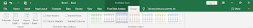
Design Tab :-The Table Tools > Design tab allows to to change many different settings that apply to Tables, including the Table's name and style. You can also convert a Table back into an ordinary Range using this tab and quickly create Pivot Tables and Slicers. 

Subtotal:- The Excel SUBTOTAL function returns an aggregate result for supplied values. SUBTOTAL can return a SUM, AVERAGE, COUNT, MAX, and others  and SUBTOTAL function can either include or exclude values in hidden rows. Get a subtotal in a list or database.

Grand Totals:- Grand Total for a range of cells Select the range of cells, and the blank row below the range, and the blank cells in the column to the right (cells A1:D5 in the example below) Click the AutoSum button on the Ribbon's Home tab. A SUM formula will be automatically entered for each Total.

Report Layout:- In Excel, Pivot tables have a defined basic structure, called a Report Layout (Form). In a new installation of Excel, pivot tables are in Compact Layout by default. See how to change to Outline or Tabular layout, and compare the features of each layout type.

Blank Rows:- Begin by selecting your data including the blank rows.

Open the Go To Special dialog by following HOME > Find & Select > Go To Special in the ribbon.

Select the Blanks option.

Click OK to apply your selection.

Row Headers:- Can show and Hide 

Column Headers:- Can Show and Hide 

Banded Row :- Can Show and Hide

Banded Column :- Can Show and Hide

Pivot table Style:- Click Design, and then click the More button in the PivotTable Styles gallery to see all available styles.Pick the style you want to use.If you don’t see a style you like, you can create your own. Click New PivotTable Style at the bottom of the gallery, provide a name for your custom style, and then pick the options you want.